This page contains a list of the known issues when using SpreadsheetConverter to convert Excel spreadsheets to live, calculating web pages.
All our files and computers are scanned for malware at all stages of production using the latest versions of industry-standard Internet security software which is updated automatically. All files available from our Download page are free of known malware. If your Internet Security software is flagging any part of our software as malicious, we urge you to contact us immediately. We are aware that e2o2.exe or ViewManager.exe sometimes get a “suspected” status, but so far these have all been false alarms. Read more on the help page for download and installation.
In 2015 we introduced an offline forms feature built on a web standard called AppCache that is now being deprecated. We want you to be aware that depending on your web browser, AppCache-based offline forms may cease to work at some point in the future.
Our developers are investigating a new implementation. If and when such an implementation appears, you will need to upgrade to the then current version of SpreadsheetConverter and use it to re-convert your offline forms to use the new functionality.
Please contact our help desk if you have any questions regarding the future support for offline forms in SpreadsheetConverter.
When you insert a new row in Excel, the default behavior is that certain properties are copied from the row above it.
In the example below, we are inserting a new row below row 23.
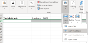
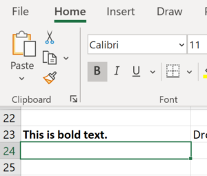
After we have inserted a new row 24, can see in A24 that the Bold font style attribute was copied from A23.
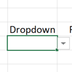
If we insert a new row below a dropdown menu, cell B24 below the dropdown in A24 also becomes a dropdown menu, as you can see from the small handle.
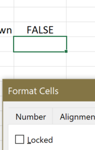
C24, the cell below the checkbox in C23, apparently did not become a checkbox. But something else happened to it, that is not easily recognized. Since C23 was unlocked, C24 quietly inherited the Unlocked attribute, which makes it an input cell if you use the Unlocked method of designating input cells.
Conclusion: Whenever you insert a new row in an Excel spreadsheet, some cell attributes will be copied from the cells in the row above the inserted row. You can try to avoid this by always selecting a row below an apparently empty row, but you may still run into issues because many “invisible” cell attributes like Bold and Unlocked remain even after the cell’s contents are deleted, and will be inherited by the new row without any visual feedback.
This is how Excel is designed, and there is nothing that SpreadsheetConverter can do about it.
Windows 10 version 1903 introduced an error that caused the Excel task pane to stop working. The most apparent issue is that you cannot type anything into text fields in the task pane.
We have developed a circumvention for this problem. If you are affected by this error in Windows you should update to SpreadsheetConverter version 10.3 or later, or use a different version of Windows that doesn’t have the error.
As Excel develops, new features are added that may be incompatible with old display drivers. This may result in apparent formatting errors.
In some systems, you may get a truncated display where some parts of the window are obviously missing or incomplete. The solution is to use the Optimize for compatibility setting described below.
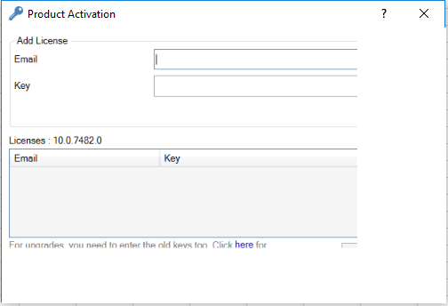
Many modern tablets and laptops have displays with much higher resolution than their predecessors. Some people refer to this as having “a high dots-per-inch ratio”, or just “high DPI”. Excel gradually gets support for such “retina” screens, but you may still see scaling issues for add-ins like SpreadsheetConverter, especially when Excel is used with two or more monitors having different resolutions.
In some Excel versions, the text in the task pane may appear to be magnified and not proportional to the rest of the content on the screen.
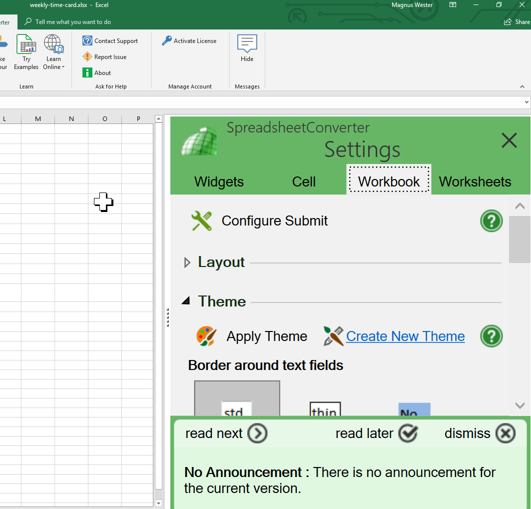
Other symptoms of these scaling issues are:
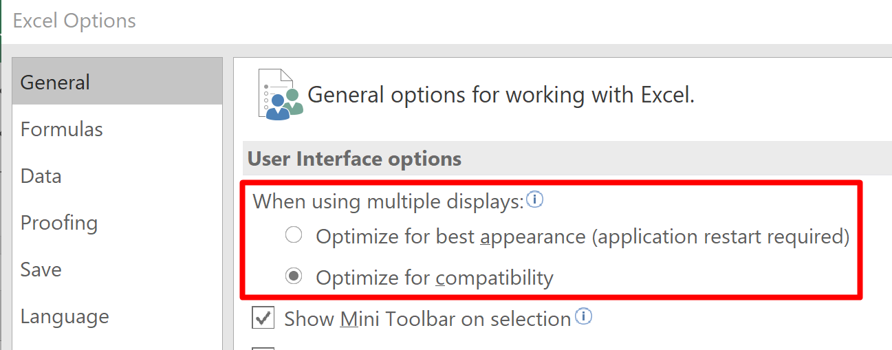
There is a simple circumvention for these problems. In Excel, go to File > Options > General > User interface options and select Optimize for compatibility.
When using the Optimize for compatibility setting, Excel gets better at handling multiple screens with different resolutions. As you can see in the screenshot below, the SpreadsheetConverter task pane is now proportional to the rest of the screen.
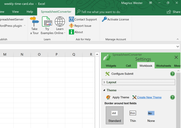
Excel does not permit add-ins like SpreadsheetConverter to control the display scaling themselves. If your version of Excel doesn’t provide the compatibility mode for multiple displays, it will not properly support multiple displays with different resolutions, and you may see scaling issues like the ones described above until you upgrade Excel.
When we designed SpreadsheetConverter we wanted to allow for extremely large spreadsheets, and still provide exceptionally fast response times on slow hardware. This forced us into a few minor compromises, of which one was that if you ever assign a text value to a cell, it is always treated like text. When you reference such a cell in your spreadsheet, it always returns a text string, even if this string only contains numbers.
In spreadsheets that you intend to use with SpreadsheetConverter, you should clearly separate numeric variables from all other variables and never assign them any value that is not numeric.
=IF($E2=0, "Error", ROUND(0.8/$H2,2))
SpreadsheetConverter will see that the formula may return the text Error and internally defines the cell as text, introducing the problems described above. To avoid this from happening, divide the functionality into two cells, one with the numeric value
=ROUND(0.8/$H2,2)
And another with the error indication
=IF($E2=0, "Error", "")
If you really need the error message to appear in the cell, perhaps for a table, you may be able to use a custom number format. A custom number format can have up to four sections of code, separated by semicolons. These code sections define the format for positive numbers, negative numbers, zero values, and text values, in that order.
<POSITIVE>;<NEGATIVE>;<ZERO>;<TEXT>
This allows you to display error messages instead of the cell contents for values that are positive when they shouldn’t be, or negative, or zero, or have a string value.
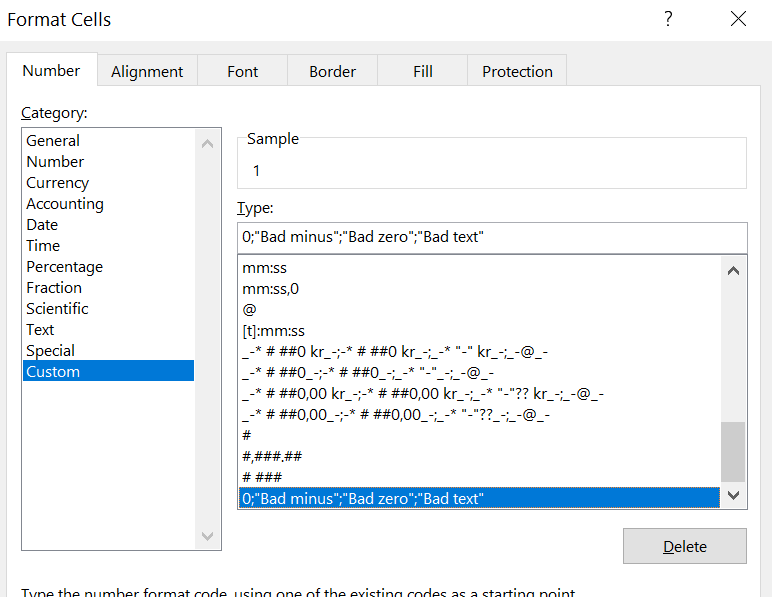
0;"Bad minus";"Bad zero";"Bad text"
The custom cell format above will only display positive numbers. All other values will be displayed as an error message. You define custom cell formats in the Format Cells dialog:
When you want to test if a numeric cell has no value, the correct way is to use a formula like
=IF(A1=0,"Empty", A1)
If you haven’t assigned any value to A1 yet, the formula above will fail, because SpreadsheetConverter regards empty cells as text strings, i.e. A1=””, and so the test will fail because A1<>0.
The obvious circumventions are:
If you really, really must have a cell that contains both text and numbers, a safe test for it being empty is
=IF(OR(TRIM(A1)="",A1=0),"Empty",A1)
Another numerical/character problem that can be really challenging is zero suppression, which just happens to be the next topic.
A common situation when cells may be forced to store both numbers and text (read more above) is zero suppression, where an otherwise numeric cell is set to blank if it is zero. Look at this worksheet for example:

If there are many numbers on the screen, and many of them are zeroes, it can be hard to quickly grasp what a table is showing. Now look at what happens when we suppress the zeroes:

Many tables become much easier to read if we remove redundant information.
Inexperienced Excel users may try to suppress the zero values using an IF clause:
=IF(sum(jan_mon_1:jan_mon_5)<>0;sum(jan_mon_1:jan_mon_5);"")
This solves a small problem in a clumsy way, but also introduces a much worse problem – it is storing string values in numeric cells. Not only will this impact performance, it also risks introducing errors if non-numeric values are later used in calculations.
A better solution? Excel has many powerful cell formatting options. Get to know them, learn how to use them, and you will have much less need for circumventions like the if clause above. For numeric fields, a “0” in the formatting template is used to show the corresponding digit even if it is a zero, and “#” to show the number only when it is not zero. Zero suppression is built into Excel!
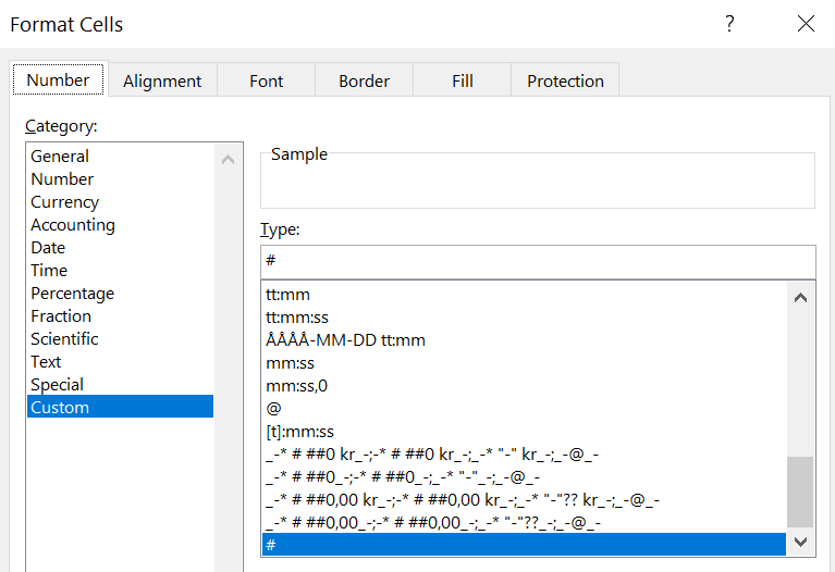
In the spreadsheet in the example above, we used the “#” custom format to suppress all the zero values in the table. It is a simple solution, but it may run into problems with currency symbols, thousand separators, and zero separators. If you want your numbers to be formatted like this:
$11,256.42
the “#” trick won’t help you, but Excel offers other ways to solve this. A custom number format can have up to four sections of code, separated by semicolons. These code sections define the format for positive numbers, negative numbers, zero values, and text values, in that order.
<POSITIVE>;<NEGATIVE>;<ZERO>;<TEXT>
You can use any advanced numeric formatting you like in the <POSITIVE> and <NEGATIVE> sections and then simply leave the <ZERO> section empty.
You can even use these code sections to create the following custom default cell format that can be used for all cells in a spreadsheet:
General;General;;@
If you apply this format to all cells in a spreadsheet, you will suppress all the zero values in all cells that don’t have their own number format set for them. All other text or numbers will have the same default formatting that they usually have.
If you like the idea, make it a habit to always apply this custom default cell format to all cells in new spreadsheets!
A common problem in Excel is that it may not show you the true, entire numeric value of a cell. For example, if you enter the formula
=1/3
into cell A6, it will typically display as 0.333333. But the value actually has an infinite number of threes. So the statement
=IF(A6=0.333333, True, False)
will evaluate as False. Also, most computers actually perform decimal calculations as their equivalent binary calculations. This inherent approximation may lead to differences in precision, e.g. that a cell ends up with a value of 0.45000001 when you were expecting it to contain exactly 0.45. So, instead of the formula above, you should consider using
=IF(ABS(A6-0.333333) < 0.000001, True, False)
The same thing happens if you want to evaluate if a value is less than or greater than another value. If you get unexpected True situations using
=IF(A5 > A6, True, False)
it may be because one of the cells contains 0.45 but the other 0.45000001. To exclude this special case – where you prefer to consider the cells to be equal – use this formula instead:
=IF(AND(ABS(A5-A6) > 0.000001, A5 > A6), True, False)
If the numbers are close enough, the first part of the AND statement will not be True, and so A5 will not be considered greater than A6. You must use a “proximity constant” that is relevant for the numbers you are actually processing, in particular if you expect the cells to contain extremely high or low values.
This issue requires you to know what version of Excel you are using. This information is available on the File > Account screen. 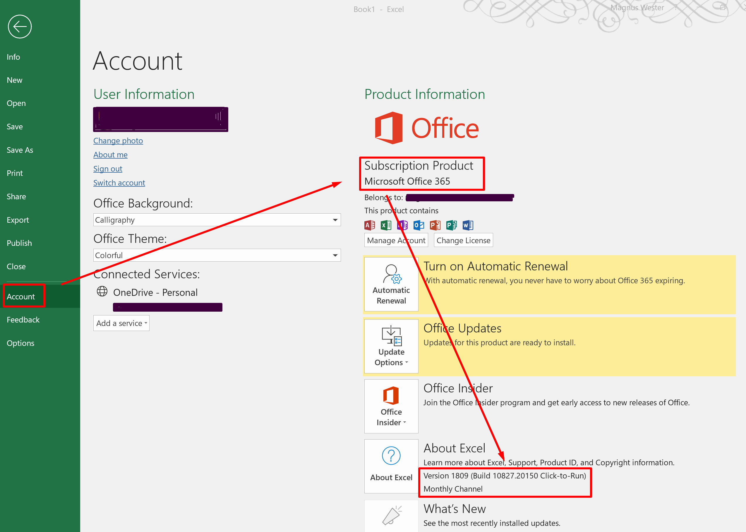 In Excel 365, version 1810, Microsoft introduced Threaded Comments. The new feature also became available in Excel 2016 version 16.17. With threaded comments, you can discuss a value or formula with other users of the same spreadsheet, just like in a chat or e-mail conversation. Notice the Reply… field in the screenshot below.

The old comments are now referred to as Notes. Notes look and work just like Comments have worked before.
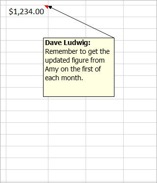
SpreadsheetConverter supports Comments from previous versions of Excel, and Notes from Excel version 1810 or 16.17, or later. If you use threaded comments in a spreadsheet that you convert with SpreadsheetConverter, the threaded comments will not be visible in the converted web page.
For your spreadsheet to convert gracefully into a properly formatted web page, it must follow certain rules. We have documented these in a separate help page about the restrictions for spreadsheet file name, size and content.
If you start a conversion and the progress bar seems to get stuck around 32%, you may be using conditional formatting on a very large cell range, e.g. an entire column. This problem is easily solved, just apply conditional formatting to only those cells that actually contain data.
When the conversion is complete, you may be shown a QR code to scan with your mobile device. If the QR code doesn’t appear automatically, you can open the History List and scan it from there. If the web page doesn’t appear in your mobile device when you scan the barcode, and you get messages saying the website is unavailable, impossible to connect to or doesn’t respond, you may need to add an exception to the Windows Firewall. Read more in the online help for Instant Testing.
New Google Maps may not appear as expected on your website. You get an error message saying Oops! Something went wrong. You likely have a problem with the Google Maps API key you use to show maps. Read the instructions on how to solve this.

When a user with the Firefox web browser presses Submit on a form that contains a chart, and you are using the Advanced Submit Service to deliver the submitted form also in PDF format, the user may get the following error message from Firefox:  The process of preparing the PDF file is partially taking place in the browser, and on slower computers the required processing may take so long that it exceeds the built-in script time-out in Firefox. The best way to verify this is to test the form with a different web browser. If the form can be submitted without errors using a different browser, you have the situation described above. The simplest solution is just to press Continue if the message appears after submission of a form. If the message becomes a problem you may suggest that the user reads Mozilla’s help page on how to increase the script time-out in Firefox to 20 seconds. Increasing the time-out has no negative effect except that it takes slightly longer for Firefox to detect other situations when a script has stopped responding – but this is not a common problem.
Our Free and Advanced e-mail services run on secure web servers, where incoming form submissions are saved. For each new form we receive on your behalf, we send an e-mail to one or more e-mail addresses designated by you, with the contents of the submitted form. E-mail is built on a store-and-forward architecture, and in the worst case, an e-mail from our server may have to pass multiple servers before it reaches its recipients. The e-mail infrastructure is beyond our control and there is simply no way for us to guarantee that you will get all the e-mails we send you. With the Advanced Submit Service, you get a personal login to our forms database. We recommend that you periodically use this login to monitor our server manually for new form submissions, in case the corresponding e-mails have been discarded by the e-mail infrastructure. The risk of losing e-mails increases when you use File Attachments. We recommend that you use our Secure Delivery feature to have the e-mail contain just a link to the form instead of the form’s full contents with attachments.
The e-mail we send you for a submitted form uses industry-standard formatting and markup. Some e-mail clients may not provide full support for current standards. In this case, hidden sheets may be visible in the e-mail, the formatting may not be perfect etc.