This is the Online Help page for the dynamic dropdown menu widget in SpreadsheetConverter.
The purpose of the Dynamic dropdown widget is to make it easy to create a dropdown menu where the options are controlled from the spreadsheet and can be changed by a formula. If you only need a simple, static list of options, it is usually easier to use the ordinary Dropdown list widget in the Basic widgets category.
Due to the inherent complexity of the Dynamic dropdown widget, it cannot be tested in Excel. You must convert your spreadsheet to a web page to test a Dynamic dropdown menu.
The Dynamic dropdown widget operates in one of two modes, either with a one-dimensional table or a two-dimensional indexed table with lookup.
In the one-dimensional mode, you provide a list of options in a cell range in your spreadsheet. The cell range can be either row- or column-oriented, and empty cells are ignored. The widget illustrates this, with a cell range containing three choices in a row.
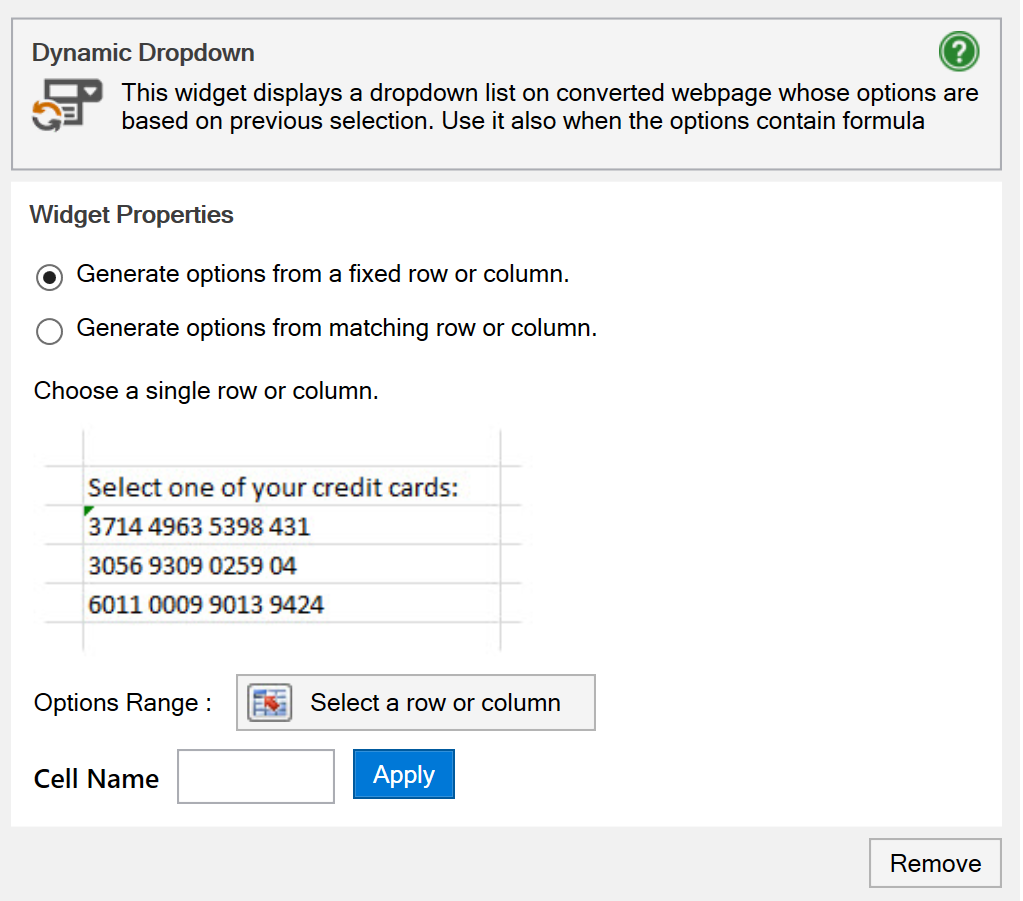
In contrast to the basic dropdown widget, however, this cell range need not contain a static list of choices.
Each cell can contain a different formula that assembles, calculates or conditionally selects content for the menu item. Here are a few examples of formulas you can expect to find in a dynamic dropdown:
=if(country_name="", city_name, city_name & ", " & country_name)
=vlookup(postcode, postcode_to_city_table, 2, FALSE)
=if(location_1_available, location_1_name, "")
Make the cell range big enough to accommodate the largest number of choices you will ever need. If you don’t need all choices there’s room for, just leave the redundant cells empty and they will be ignored when the dynamic dropdown is created.
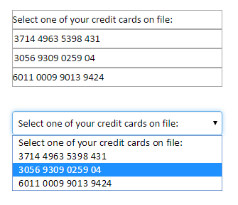
If you want to add a prompt, e.g. Select one of your credit cards on file at the top of the menu, just make it the first choice in the cell range.
There is an example of a one-dimensional Dynamic Dropdown in the tutorial for the Link Image widget
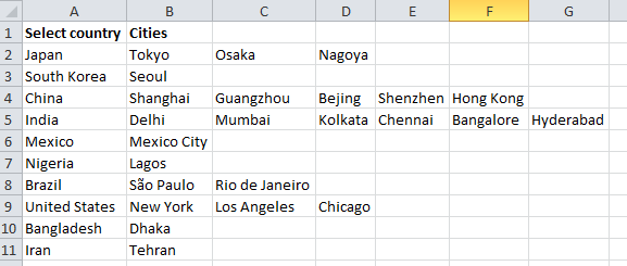
The two-dimensional mode is best explained with an example. Let’s say we want to show the world’s biggest cities per country. We create a list of countries in a column, and a list of cities in the same row as the corresponding country.
In the table below, the index is located in the first column, in cells A2:A11. For each country, there is a list of cities on the same row. For Japan, the biggest cities are Tokyo, Osaka and Nagoya, in that order.
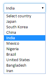
It is very easy to display this index as a country selector, using a one-dimensional dynamic dropdown. Note that we have already placed a user prompt in cell A1 at the top of the list. Just select A1:A11 in the worksheet above as the cell range to provide the choices for the one-dimensional dynamic dropdown.
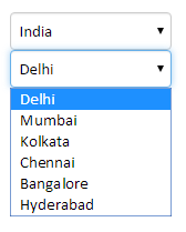
When the web page is shown in the web browser, the dropdown menu will display the user prompt Select country. In the example, the user has selected India.
When the user moves on to the second dropdown, its contents are set dynamically, depending on the country selection. For India, the choices are located in cells B5:G5 of the spreadsheet above, and the city dropdown would immediately change to look like this:
Every time you change the country in the upper dropdown menu, the appropriate cities appear in the lower dropdown menu. This can dramatically increase the speed of data entry, the accuracy and the quality of an electronic form.
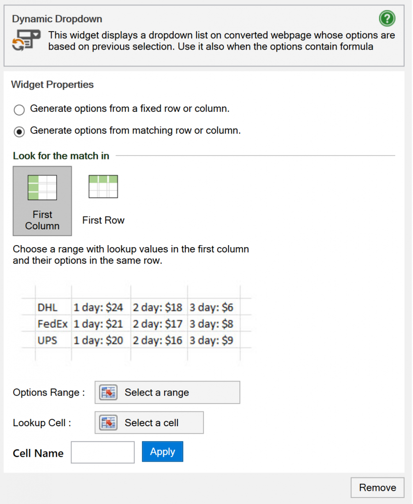
In the two-dimensional mode, you provide the cell range for an indexed, two-dimensional table in the Options Range setting.
Do you want the index in a column, with the options in the cells to the right, as in the country/city example above? We call this the (Index is in the) First Column setting. If the index is longer than the longest list of choices, this may be the easiest layout to work with.
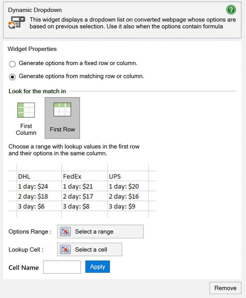
If the index is short but the number of options can be long, it may be more convenient to use the (Index is in the) First Row setting. In this setting, the top row of the Options Range contains the index, with the menu choices for each key in the cells below it.
A separate Lookup Cell is matched against the index. In the “major cities” example above, the Lookup Cell is the one-dimensional dropdown used to set the country. It can contain the value Japan. When the Lookup Cell matches a key in the index, the dynamic dropdown menu is populated with all the menu choices for that key. For Japan, those choices are Tokyo, Osaka and Nagoya.
You can use many types of widgets for the Lookup Cell, e.g. radio buttons, sliders and even check boxes.
The value for the Lookup Cell doesn’t have to come from a widget, any cell in the spreadsheet can be used for lookup.
Dynamic dropdowns take their choices from a cell range in the spreadsheet. You may fill this cell range with any kind of content and change it depending on other cells.
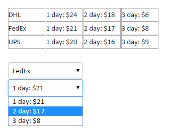
As an example, you may know the origin, destination, dimension and weight for a pending shipment. Using this information, your spreadsheet dynamically assembles a price list from three couriers. All the user has to do is to determine the urgency and pick the best choice.
Why stop at only two dimensions?`You can use one menu for a country, a second for postal codes per country, and a third for cities per postal code. And a fourth for streets per city! There is no technical limit to the number of levels or “dimensions” in such a menu structure.
You can create all the menu choices in the Options Range using the same programming techniques as we described for the one-dimensional dropdown above.